Checking interpolation of phonon modes
In this tutorial, we will try to plot the phonon modes and its derivatives as functions of volume.
Load the configuration and run the Calculator
Same as performing calculations programatically, we need to load the qha-cij calculator first.
[1]:
import cij.core.calculator


calculator = cij.core.calculator.Calculator("_attachments/plotting/config.yml")
/Users/chazeon/Documents/Projects/qha-cij-2/cij/core/phonon_modulus.py:88: RuntimeWarning: divide by zero encountered in true_divide
  return  h_div_k * (self.freq_array[nax,:,:,:] / self.t_array[:,nax,nax,nax])
/Users/chazeon/Documents/Projects/qha-cij-2/cij/core/phonon_modulus.py:88: RuntimeWarning: invalid value encountered in true_divide
  return  h_div_k * (self.freq_array[nax,:,:,:] / self.t_array[:,nax,nax,nax])
/Users/chazeon/Documents/Projects/qha-cij-2/cij/core/phonon_modulus.py:96: RuntimeWarning: overflow encountered in exp
  return self.Q ** 2 * numpy.exp(self.Q) / (numpy.exp(self.Q) - 1) ** 2
/Users/chazeon/Documents/Projects/qha-cij-2/cij/core/phonon_modulus.py:96: RuntimeWarning: overflow encountered in square
  return self.Q ** 2 * numpy.exp(self.Q) / (numpy.exp(self.Q) - 1) ** 2
/Users/chazeon/Documents/Projects/qha-cij-2/cij/core/phonon_modulus.py:96: RuntimeWarning: invalid value encountered in true_divide
  return self.Q ** 2 * numpy.exp(self.Q) / (numpy.exp(self.Q) - 1) ** 2
/Users/chazeon/Documents/Projects/qha-cij-2/cij/core/phonon_modulus.py:92: RuntimeWarning: overflow encountered in exp
  return self.Q / (numpy.exp(self.Q) - 1)
/Users/chazeon/Documents/Projects/qha-cij-2/cij/core/phonon_modulus.py:92: RuntimeWarning: invalid value encountered in true_divide
  return self.Q / (numpy.exp(self.Q) - 1)
Plotting the interploated phonon modes and its derivatives
To plot phonon modes, we could use the ModePlotter module.
To use this module, we mport it first, and create a ModePlotter object plotter and initialize it with the Calculator we prepared above. With the plotter we can easily plot the interpolated mode frequency \(\omega_{qm}(V)\), Grüneisen parameter \(\gamma_{qm}(V)\) and \(V\partial\gamma_{qm}/\partial V\) with it.
[2]:
from cij.plot import ModePlotter
from matplotlib import pyplot as plt

plotter = ModePlotter(calculator)
The method used for plotting these parameters as a function of volumes (in Å\(^3\)) is plot_modes, the first parameter is the pyplot handle or an Matplotlib Axes. Two other optional parameters controls the behavior of the plotting method
ncontrols is the order of derivatives, wheren = 0(default) plots interpolated mode frequency \(\omega_{qm}(V)\), and additionally scatters the uninterpolated phonon frequency data as in the QHA input with it.n = 1plots Grüneisen parameter \(\gamma_{qm}(V)\)n = 2plots \(V\partial\gamma_{qm}/\partial V\)
iqcontrols the \(q\) point to plot on, usually,iq = 0means you are plotting all the modes at \(\Gamma\) point.
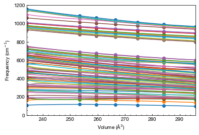
In the following 3 pieces of codes, I plot mode frequency \(\omega_{qm}(V)\), Grüneisen parameter \(\gamma_{qm}(V)\) and \(V\partial\gamma_{qm}/\partial V\) respectively at \(\Gamma\) point respectively.
[3]:
plt.figure()

plotter.plot_modes(plt, n = 0)

plt.ylim(0, 1200)
plt.xlim(min(plotter.volumes), max(plotter.volumes))
plt.xlabel("Volume (Å$^3$)")
plt.ylabel("Frequency (cm$^{-1}$)")

plt.show()
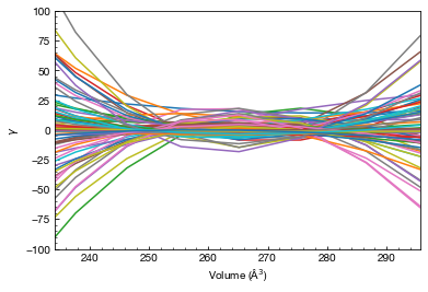
[4]:
plt.figure()

plotter.plot_modes(plt, n = 1)

plt.ylim(-100, 100)
plt.xlim(min(plotter.volumes), max(plotter.volumes))
plt.xlabel("Volume (Å$^3$)")
plt.ylabel("$\\gamma$")

plt.show()
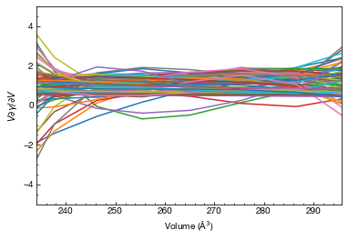
[5]:
plt.figure()

plotter.plot_modes(plt, n = 2)

plt.ylim(-5, 5)
plt.xlim(min(plotter.volumes), max(plotter.volumes))
plt.xlabel("Volume (Å$^3$)")
plt.ylabel("$V\\partial\\gamma/\\partial V$")

plt.show()